All 15 résultats
Trier par
-
Drawing_Maps_VisualAnalytics_Week14_NEC_Solved
- Examen • 11 pages • 2023
- €10,02
- 2x vendu
- + en savoir plus
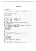
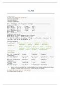
1. pipe the election data through the select() function to pick out the following columns - state, total_vote, r_points, pct_trump, party, census. Pipe that through sample() to see the first five rows. 2. Create a state level dotplot of election data except the District of Columbia faceted by region. Colorize the dots by party and insert a vertical line dividing the parties, scale the x axis from -30 to +40, put the states on the y axis and label each facet by region and the entire set by "Poi...
-
Working_with_Models_VisualAnalytics_Week9_NEC_Solved
- Examen • 8 pages • 2023
- €10,02
- 2x vendu
- + en savoir plus
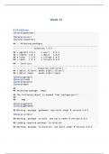
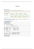
1. Using the gapminder data, create a plot comparing log(gdp PerCa with Life Exp and show three different smoothers in three different colors with a legend showing each smoother type. 2. In a paragraph compare and contrast the smoother types. LOESS, Cubic Spline, and OLS 3. Look at the gapminder data with str() 4. Create a linear model of the gapminder data with life expectancy as the target of a multifactor model built from gdpPercap, pop, and continent. Store it in a variable called ...
-
Plotting_Text_VisualAnalytics_Week7_NEC_Solved
- Examen • 10 pages • 2023
- €10,02
- 1x vendu
- + en savoir plus
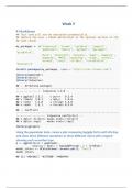
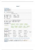
1. produce a scatterplot of the by_country data with the points colored by consent_law 2. Using facet_wrap() split the consent_law variable into two panels and rank the countries by donation rate within the panels 3. Use geom_pointrange() to create a dot and whisker plot showing the mean of donors and a confidence interval. 4. Create a scatterplot of roads_mean v. donors_mean with the labels identifying the country sitting to the right or left of the point 5. load the ggrepel() library 6. ...
-
Refining_your_Graphs_VisualAnalytics_Week14_NEC_Solved
- Examen • 6 pages • 2023
- €10,02
- 1x vendu
- + en savoir plus
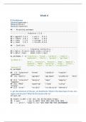
1. look at the first six rows of the asasec dataset 2. plot members v revenue for 2014 in a scatterplot with a confidence interval 3. switch from loess to ols and add the Journal variable 4. show the first six rows of studebt 5. create a faceted comparison of the two distributions - percent of all borrowers and Percent of all balances to show how student loan debt is distributed. 6. Compare this pair of graphs to the pie charts in figure 8.24 Which visualization do you find it easier to ma...
-
Using_our_Tools_VisualAnalytics_Week8_NEC_Solved
- Examen • 10 pages • 2023
- €10,02
- 1x vendu
- + en savoir plus
1. Return to the visualization for Presidential Elections: Popular and Electoral College margins, subset by party, and use that to add color to your points. 2. Recreate figures 5.28 using functions from the dplyr library. 3. Using gss_sm data, calculate the mean and median number of children by degree 4. Using gapminder data, create a boxplot of life expectancy over time 5. Using gapminder data, create a violin plot of population over time
-
Drawing_Maps_VisualAnalytics_Week13_NEC_Solved
- Examen • 11 pages • 2023
- €10,02
- 1x vendu
- + en savoir plus
1. pipe the election data through the select() function to pick out the following columns - state, total_vote, r_points, pct_trump, party, census. Pipe that through sample() to see the first five rows. 2. Create a state level dotplot of election data except the District of Columbia faceted by region. Colorize the dots by party and insert a vertical line dividing the parties, scale the x axis from -30 to +40, put the states on the y axis and label each facet by region and the entire set by ...
-
Grouped_Analysis_and_List_Columns_VisualAnalytics_Week11_NEC_Solved
- Examen • 7 pages • 2023
- €10,02
- 1x vendu
- + en savoir plus
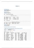
1. Take a slice of the gapminder data showing only 1977 2. create a linear model of with lifeexp being the target of the log of gdpPercap. Save it in a variable called fit and show the summary. 3. Group the entire data set by continent and year, pipe it through the nest() function and store it in a variable called out_le. 4. The result will be a tibble of columns of data and columns of tibbles called list columns with data in them. 5. Use the filter() and unnest() functions to see Europe 1...
-
Plotting_Marginal_Effects_VisualAnalytics_Week12_NEC_Solved
- Examen • 7 pages • 2023
- €10,02
- 1x vendu
- + en savoir plus
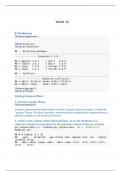
1. load the margins library 2. create a new column called called polviews_m to use Moderate as a reference category using relevel on the polviews column of the gss_sm data. 3. use glm() to create a model called out_bo using logistic regression of polviews_m with sex and race showing an interaction glm(obama~ polviews_m + sex*race, family = "binomial", data = gss_sm). 4. use summary() on out_bo to see what the results look like 5. calculate the marginal effects of each variable and sto...
-
The_broom_Package_VisualAnalytics_Week10_NEC_Solved
- Examen • 9 pages • 2023
- €10,02
- 1x vendu
- + en savoir plus
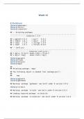
1. load the broom library 2. use tidy() on the out dataframe to produce a new dataframe of component level information. Store the result in out_comp. 3. round all the columns to two decimal places using round_df(). 4. Produce a flipped scatter plot of Term v. Estimate 5. Produce a new tidy output of out including confidence intervals. Store it in a variable called out_conf after rounding the dataframe to two decimals. 6. Remove the intercept column and the term continent from the label and ...
-
Building_Layered_Visualizations_VisualAnalytics_Week6_NEC_Solved
- Examen • 16 pages • 2023
- €10,02
- + en savoir plus
1. get the structure of the gss_sm dataframe. What is the data type of race, sex, region and income? What do the levels refer to? 2. create a graph that shows a count of religious preferences grouped by region 3. turn the region counts in percentages 4. use dodge2() to put the religious affiliations side by side within regions 5. show the religious preferences by region, faceted version with the coordinate system swapped 6. using pipes show a 10 random instances of the first six columns in...